Built for analysts and researchers · macOS download coming soon
THE WORK IS VISIBLE
Every connection is a step you can inspect.
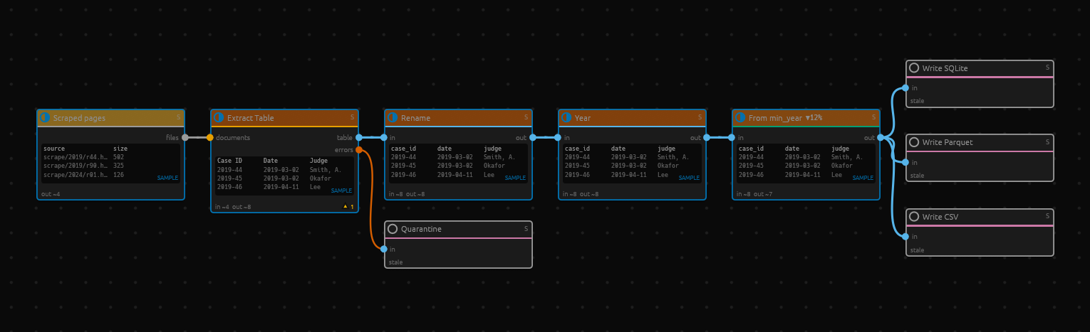
IOPIPE CANVAS · ROW PREVIEWScourt_rulings.iopipe
SAVE THE METHOD, NOT JUST THE OUTPUT
A clean dataset is useful. A repeatable path to it is better.
When the next survey wave lands or another batch of files arrives, the work shouldn’t start over. In ioPipe, your preparation, analysis, and exports stay connected in a saved pipeline.
HOW IT WORKS
Build it. Check it. Run it again.
Work visually, with the detail close at hand.
01 Connect the steps
Bring in your files, then connect nodes to clean, join, and analyze them. Branch the same data into a table, a chart, or several export formats.
02 See what changed
Inspect sample rows at each step before running the full dataset. Route extraction errors into a separate output so they’re available for review.
03 Keep what works
Save the whole graph as an .iopipe file. Reuse it with new inputs, share the method, or run it from the command line.
ONE CONNECTED WORKFLOW
From “what’s in these files?” to “here’s what we found.”
Keep the route from source to result in view.
↳ Make messy data usable
Extract HTML tables, clean text, handle missing values, and join datasets. Read survey formats including SPSS, SAS, and Stata.
↗ Follow through to the answer
Score survey scales, compare groups, and fit regression models. Turn the results into charts or maps in the same graph.
✳ Give AI a defined job
Classify reviews or extract fields with a configured local or hosted model. Cache responses and replay them as you refine downstream steps.
⇄ Take the work with you
Export datasets to CSV, Parquet, SQLite, and more. Save charts as SVG, PNG, or PDF. Share the pipeline alongside the result.
Built-in MCP support. Connect a compatible AI assistant through the Model Context Protocol (MCP) to build and edit pipelines, preview sample rows, and start runs.
REAL WORKFLOWS, CONCRETE OUTPUTS
Start with a question. End with something useful.
01 / DATA EXTRACTION
Turn court pages into a dataset
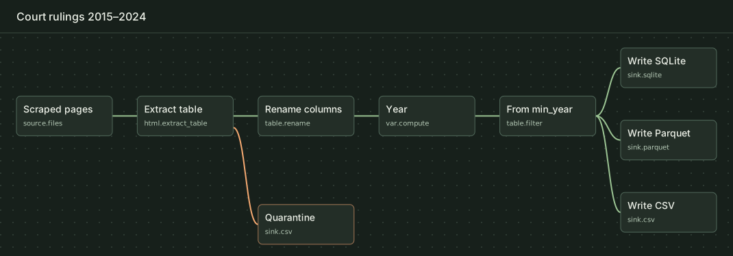
Read scraped HTML, extract ruling tables, rename the columns, and filter by year. The same cleaned data goes to CSV, Parquet, and SQLite. Pages without a matching table go to a quarantine file.
The sample run exported seven rulings and flagged one page with no matching table.
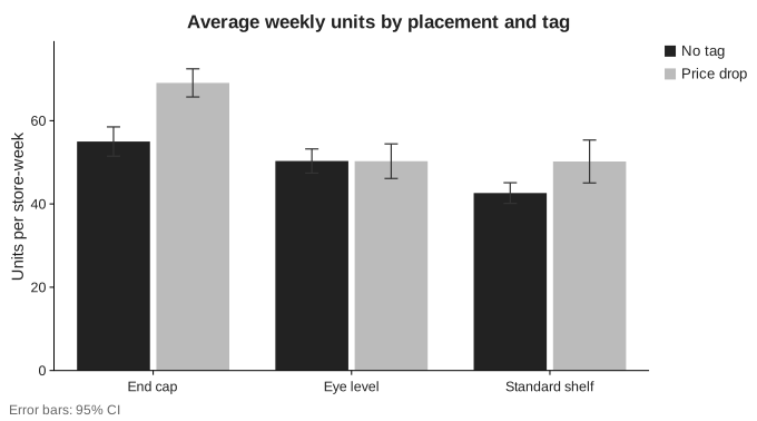
Aggregate weekly iced tea sales to the store level. Then use a two-way ANOVA to test whether the tag’s effect depends on shelf placement, and chart the six group means.
In the simulated data, end-cap displays averaged 69 units per week with a tag and 55 without. Eye-level displays averaged about 50 either way.
Interaction chart exported by ioPipe
03 / GEOSPATIAL ANALYSIS
Map where the 2024 polls missed
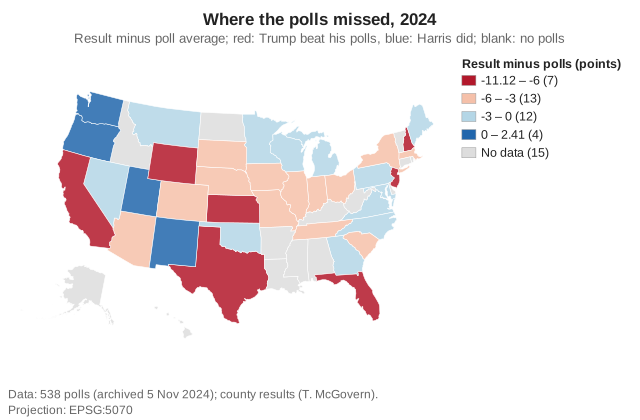
Aggregate archived 538 polls and county election returns to the state level. Join the results to Census state boundaries and map the gap between the final poll average and the result.
All ten states with at least ten late polls shifted toward Trump relative to their poll averages in this run.
Polling error map exported by ioPipeMore example projects
Brand tracking — combine survey waves, score scales, and export a codebook and SPSS file.
Satisfaction drivers — use factor analysis and regression to study satisfaction and score churn risk.
Campaign test — validate a send log, join CRM records, and compare email offers by segment.
App redesign — test how an app redesign affects spending and whether the indirect effects vary by age.
Customer reviews — extract review fields from HTML and compare human and model topic labels. AI steps require a configured model.
Product reviews — classify real reviews by sentiment using a local model adapter. This example requires local model setup.
Store catchment — find the nearest store, group customers by distance, and map areas with weak coverage.
UNDER THE HOOD
Simple to follow. Plenty to work with.
Explore the built-in tools for preparation, analysis, visualization, and export.
Explore the full node catalog, MCP, and Python options
Built-in node catalog
Expand a category to see its nodes. Each entry shows the name from the app and what the node does.
File discovery and input readers 5
FilesFind files in a folder using filename patterns.
Read CSVCombine CSV or TSV files with matching headers into one table.
Read SASImport SAS data and transport files with variable labels and formats.
Read SPSSImport SPSS data with value labels, missing-value codes, and case weights.
Read StataImport Stata data with variable labels, value labels, and date formats.
HTML parsing and extraction 3
Extract FieldsPull text or attributes from HTML using CSS selectors.
Extract TableTurn HTML tables into rows and match columns by their headers.
Parse HTMLDecode HTML pages using their detected character encoding.
Column transformations 18
Automatic RecodeAssign numeric codes to distinct values and keep the originals as labels.
Clean TextTrim whitespace, strip HTML, and treat placeholders like N/A as missing.
Compute VariableCreate or update a column using a SQL expression.
Count Values within CasesCount how many selected columns match a value or range in each row.
Date & TimeParse dates, extract date parts, and calculate or add time intervals.
Dummy CodingCreate a binary indicator column for each category.
LagCopy values from earlier rows, optionally within each group.
Lookup / Map ValuesReplace values using a lookup table, such as a codebook.
PseudonymiseHash IDs, remove direct identifiers, or reduce the precision of identifying fields.
RecodeReplace individual values or ranges according to rules you define.
RenameRename columns individually or with a pattern.
Replace Missing ValuesFill gaps with a mean, median, fixed value, or last valid value.
Reverse ScoreReverse the direction of a rating scale while preserving missing values.
Scale ScoreSum or average survey items that meet a minimum response count.
Select / Drop / ReorderChoose which columns to keep and how to order them.
StandardizeRescale values using z-scores, min–max scaling, or the median and interquartile range.
String FunctionsChange case, replace text, or extract and combine parts of strings.
Visual BinningGroup numeric values into labeled intervals.
Row operations 7
Add Row NumberNumber rows across the table or within each group.
ExplodeTurn each item in a list or delimited field into its own row.
Identify Duplicate CasesFlag rows with duplicate keys or keep one row per key.
Limit / RangeKeep a fixed number of rows, with the option to skip rows first.
SampleDraw a repeatable random sample by fraction or exact row count.
Select CasesKeep or flag rows that match a SQL condition.
Sort CasesOrder rows by one or more columns while preserving the order of ties.
Joins, aggregation, and reshaping 7
AggregateCalculate group totals, averages, counts, and other summaries.
JoinCombine two tables by matching key columns.
Merge: Add CasesStack two tables, matching columns by name.
Merge: Add VariablesBring columns from a lookup or matching table into the original rows.
Restructure: Cases to VariablesPivot repeated rows into separate columns for each ID.
Restructure: Variables to CasesTurn groups of columns into rows and add an index to identify each group.
SQLRun a SQL query across up to three input tables.
Labels, weights, and validation 7
Apply LabelsSwap coded values for their labels or convert labels back to codes.
Define Missing ValuesMark specific values or ranges as missing for later steps.
Split FileTell later steps to calculate results separately for each group.
Validate DataCheck data against rules and flag, report, or drop rows that fail.
Value LabelsAttach readable labels to coded values, such as survey responses.
Variable PropertiesSet column labels, measurement levels, roles, and display formats.
Weight CasesChoose a column that determines how much each row counts in later analyses.
Data profiling and summaries 7
CrosstabsCompare two categorical variables using counts, percentages, and tests of association.
Data ProfileReview each column’s type, missing values, range, and common values.
DescriptivesSummarize numeric columns with counts, averages, spread, and range.
Explore / QuantilesExplore numeric distributions with medians, percentiles, and interquartile ranges.
FrequenciesCount how often each value appears and report percentages and missing responses.
Means by GroupCompare averages, standard deviations, and counts across groups.
Missing Value PatternsFind which columns have missing values and which tend to be missing together.
File, database, and report outputs 10
CodebookExport a Markdown or HTML reference for variables, labels, and missing-value codes.
Export ChartSave a chart as SVG, PNG, PDF, or Vega-Lite JSON at a specified size.
Results TableExport an APA-style results table to Word, LaTeX, HTML, or Markdown.
Save ModelSave a fitted model for sharing or prediction in another pipeline.
Write CSVExport rows to a comma- or tab-separated file.
Write JSONLExport one JSON object per row.
Write ParquetExport typed columns and variable metadata to a Parquet file.
Write SPSSExport an SPSS file with labels, missing-value codes, and case weights.
Write SQLiteCreate, replace, or append to a table in a SQLite database.
Write StataExport a Stata data file with variable labels, value labels, and formats.
Statistical tests and models 12
ANOVACompare group means across factors, test interactions, and account for covariates.
Chi-squareTest whether observed counts fit an expected distribution or whether categories are associated.
Correlation MatrixMeasure associations with Pearson, Spearman, Kendall, or partial correlations.
Linear RegressionModel a numeric outcome and estimate how predictors relate to it.
Logistic RegressionModel a binary outcome and estimate probabilities and odds ratios.
Mediation & Moderation (PROCESS)Test indirect effects and how effects vary across conditions using PROCESS models.
Multiple ComparisonsAdjust p-values to account for multiple tests.
Nonparametric TestsCompare groups or paired measurements using rank-based or sign tests.
PCA / Factor AnalysisReduce a set of variables to components or estimate underlying factors.
PredictApply a fitted model to new rows to generate predictions or factor scores.
ReliabilityAssess how consistently survey items measure a scale using alpha and omega.
t-testsTest a mean against a benchmark or compare independent or paired means.
Charts and result tables 12
Bar ChartCompare category totals, percentages, or averages with grouped or stacked bars.
Box PlotShow medians, quartiles, and outliers across groups.
Chart StyleApply consistent colors, fonts, labels, and sizing to charts.
Coefficient PlotPlot regression estimates and confidence intervals side by side.
HeatmapShow a correlation matrix or summary table as a grid of colors.
HistogramShow how numeric values are distributed across intervals.
Line / Time SeriesPlot trends across dates or numeric intervals, optionally with a moving average.
MapMake a map with up to three layers and color features by value or category.
Model DiagnosticsPlot residuals and leverage to check a linear regression fit.
Q-Q PlotCompare observed and normal quantiles to check whether data follow a normal distribution.
ScatterPlot the relationship between two numeric columns, with optional groups or a fitted trend.
Small MultiplesArrange several charts in one figure.
Geospatial processing and maps 34
Aggregate & SuppressSummarize points by area and hide results where too few records contribute.
Aggregate to AreasCount points and summarize their values within polygons or H3 cells.
Areal InterpolationTransfer values between boundary systems based on how much their areas overlap.
BufferExpand or shrink features by a specified distance.
ClipTrim lines and polygons to a boundary and discard points outside it.
DissolveMerge geometries by group and summarize their attributes.
DistanceMeasure the distance between two geometries or to a fixed location.
Explode Multi-partSplit a multipart geometry into one row per part.
Gazetteer MatchMatch place names in fields or text to an offline directory of locations.
GeocodeTurn addresses or place names into coordinates and report match scores.
GeomaskShift points by a repeatable random distance before sharing location data.
Geometry to ColumnsConvert shapes to coordinates, bounding boxes, or standard text formats.
Grid / TessellateCover an area with square or hexagonal cells for mapping and analysis.
H3 IndexAssign points or polygons to cells in the H3 hexagonal grid.
Make PointsBuild point geometries from latitude and longitude or projected coordinates.
MeasureCalculate area, length, perimeter, centroids, or other geometry measurements.
Moran's ITest whether nearby places tend to have similar values.
Nearest NeighbourFind the closest features in another layer and report their distances.
Parse GeometryRead geometry from formats such as WKT, WKB, GeoJSON, or H3 cell IDs.
Read GeoJSONImport GeoJSON features with their geometry and attributes.
Read GeoPackageLoad a feature layer and its coordinate system from a GeoPackage.
Read GeoParquetLoad geometry and attributes from GeoParquet, optionally within a bounding box.
Read ShapefileImport geometry and attributes from plain or zipped shapefiles.
ReprojectConvert geometry to a different coordinate reference system.
SimplifyReduce the number of vertices in lines and polygons for smaller files and faster maps.
Spatial FilterKeep features that lie within or intersect a chosen area.
Spatial JoinAttach attributes from another layer based on where features intersect or how close they are.
Spatial LagCalculate the weighted average of neighboring features’ values.
Spatial WeightsDefine which features are neighbors and how much each neighbor counts.
Validate & Repair GeometryCheck for geometry problems and repair, flag, or drop invalid features.
Write GeoJSONExport features and attributes as a GeoJSON collection or sequence.
Write GeoPackageSave a feature layer with its coordinate system and spatial index in a GeoPackage.
Write GeoParquetExport features to Parquet with standardized geometry metadata.
Write ShapefileExport a feature layer as an ESRI shapefile and its companion files.
AI models and coding agreement 5
AgreementMeasure how often two coders agree and where their labels differ.
EmbedConvert text to numeric vectors for similarity search or clustering.
LLM ClassifyAssign one or more predefined categories to each row with a language model.
LLM ExtractUse a language model to extract structured fields from unstructured text.
LLM PromptSend a customized prompt for each row and store the response as text or JSON.
Reusable graph inputs and outputs 2
Library InputBring data into a reusable group of nodes through a named port.
Library OutputExpose a result from a reusable group of nodes through a named port.
Model Context Protocol (MCP)
In the desktop app, open File → Connect an AI Assistant to start a local MCP server and copy its connection settings. Command-line clients can launch the server with iopipe mcp --workspace DIR.
Optional Python sidecar
Use Python reference implementations for Descriptives, Means, Frequencies, and Crosstabs during full runs. Enable it in the desktop app under Settings → Python sidecar and turn it on from the toolbar, or point the command line at your configured sidecar with iopipe run FILE.iopipe --sidecar verify.
Previews use the built-in implementation. During a full run, ioPipe falls back to the built-in node when the Python implementation declines a configuration. The node’s run statistics show which implementation ran.
BUILD ON YOUR OWN WORK
Make the next run the easy part.
ioPipe for macOS is on its way. Explore a sample workflow while the public download is being prepared.